Computing the Time-Evolution of a System

To propagate a given initial state in time, one has to change only a few parameters in the MCTDHX.inp file. To start, it's best to create a subdirectory for the propagation inside the MCTDH-X-Tutorial directory which contains the relaxation:

 cd ~/MCTDH-X-Tutorial
 mkdir propagation-double-well

. As indicated by the name, we're going to propagate the groundstate of the harmonic potential, which we computed in the previous subsection, in a double well potential. First, we copy the necessary files to the newly created directory:

 cp MCTDHX.inp libmctdhx.so analysis.inp PSI_bin CIc_bin ./propagation-double-well/
 cd propagation-double-well

. Subsequently, the input file needs to be adapted with a text-editor, i.e.,

 gedit MCTDHX.inp

. To make the program propagate the initial state in the binary data files PSI_bin and CIc_bin, the following parameters have to be adapted:

 Job_Prefactor=(0.d0,-1.d0)
 GUESS='BINR'
 Binary_Start_Time=20.0d0

as also explained in the inlined documentation in the MCTDHX.inp file and in table 3, Job_Prefactor = (0.d0, -1.d0) triggers the program to do a forward time propagation, GUESS = 'BINR' will make it read the initial state from the binary files CIc_bin and PSI_bin, and Binary_Start_Time = 20.d0 chooses the time at which the binary files CIc_bin and PSI_bin are read for the initial state. Now, in order to define the parameters specifying the propagation in the double well, we change the following variables in the MCTDHX.inp :

 Integration_Stepsize=0.0001d0
 whichpot="h+d" 
 parameter1=2.d0
 parameter2=8.d0
 parameter3=1.d0

. Integration_Stepsize=0.0001d0 specifies the initial time-step (compare table 3). The which_pot = ``h+d'' variable selects a potential which is the sum of a displaced harmonic potential and a discplaced Gaussian barrier in its center. To define the potential parameter1=2.d0 is the displacement, parameter2=8.d0 specifies the height of the barrier in the center of the parabola and parameter3=1.d0 gives the width of this barrier. Finally, we select the appropriate integrator to propagate the coeffcients' equations of motion:

 Coefficients_Integrator='MCS'

. Now the input is adjusted to start the propagation and we type

 MCTDHX

to run it and wait until it finished. After it has finished, we can get a quick visualization of the final state by typing

 mctdhx_status.sh
 gnome-open status.png

. The script mctdhx_status.sh plots the time-evolution of the fragmentation in a computation as well as a snapshot of the current density. The picture you should see is displayed in Figure 3.

Figure 3: Checking the status of an MCTDH-X computation with mctdhx_status.sh.

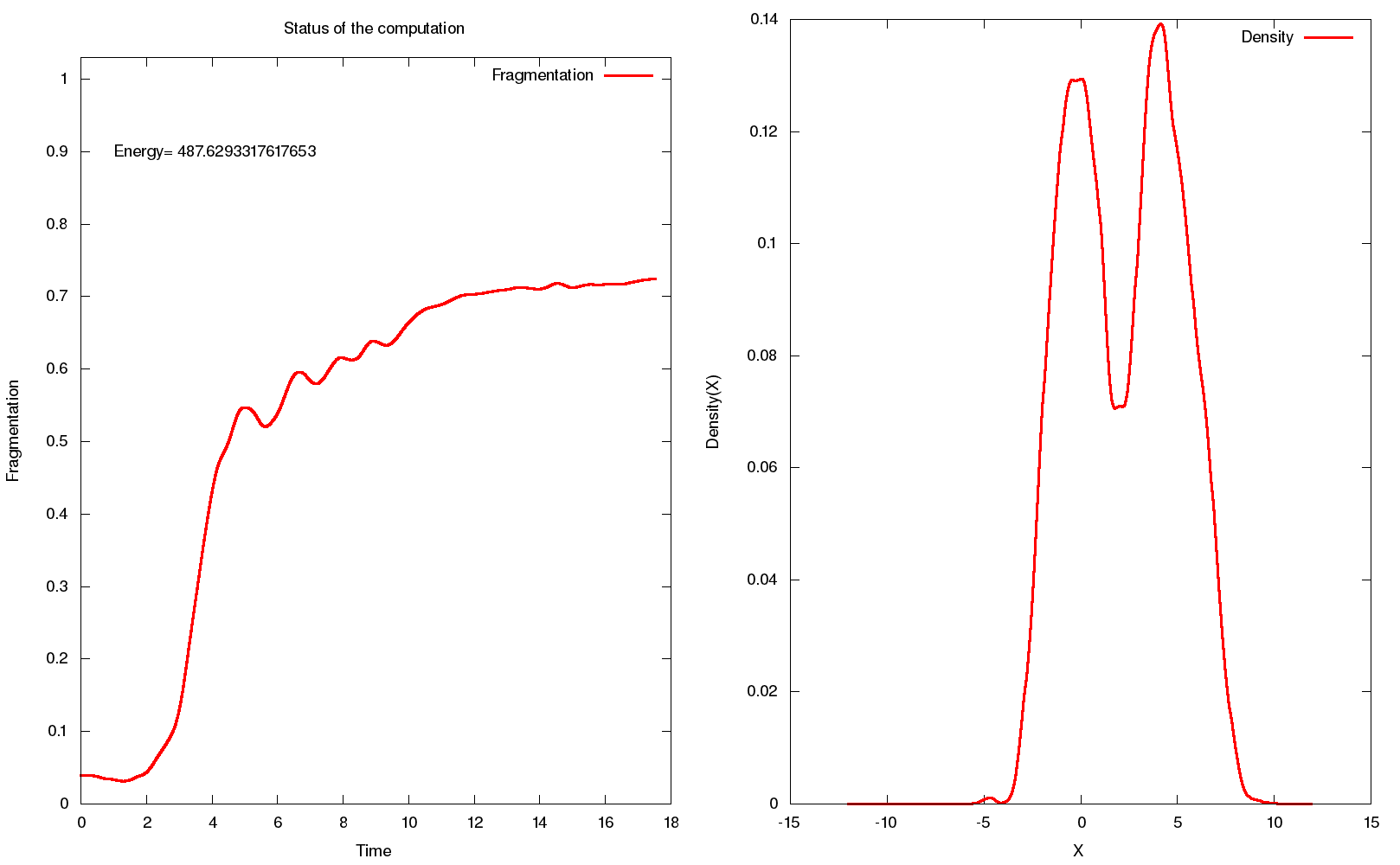The left panel displays the time-evolution of fragmentation, i.e., $1-\sum_{i=2}^M \rho_i^{(NO)}(t)$, in the system and the right panel shows a snapshot of the current density.

Finally, we could invoke several different bash-scripts to visualize the computed time-evolution as movies (cf. table 9) or simply run all available scripts with the visualization master script, like so:

 vms.sh all $PWD -7.0 9.0

(cf. also section 4.3). vms.sh automatically runs the analysis program on the data in the present directory and creates videos of the density as well as the correlation functions of the system. For reference, these are also available on the website at
http://ultracold.org/documentation.