Computing an Eigenstate by Relaxation

After the installation script has finished, you should make sure that the aliases and links are working. To do so, first type

 source ~/.mctdhxrc 
 ls $MCTDHXDIR

. Now you should see the executables MCTDHX_<compiler>, MCTDHX_analysis_<compiler> and the library libmctdhx.so. If you don't, the installation did not terminate correctly and you should check what went wrong (see the log files created in ./log/ ) and contact the developers in case you cannot find out or fix the error.

To get started, it's best to create a directory for the tutorial computations:

 mkdir ~/MCTDH-X-Tutorial
 cd ~/MCTDH-X-Tutorial

. To copy all necessary files to run the computation in this directory, we make use of the alias inpcp and libcp which copy the example inputs MCTDHX.inp, analysis.inp and the dynamic library libmctdhx.so to the current directory.

 libcp
 inpcp
 ls

. The ls command should show a list including MCTDHX.inp, analysis.inp, and libmctdh.so. With these three files, we're able to run the main and analysis programs. The default MCTDHX.inp is configured to compute the eigenstate of $N=2$ bosons in a one-dimensional harmonic oscillator potential with unit frequency and with $M=4$ orbitals. To make things a little more interesting, let's change the the number of bosons to $N=50$ by editing MCTDHX.inp and setting Npar = 50 in the System_Parameters namelist, i.e.,

 gedit ./MCTDHX.inp

. Since we're going to compute some dynamics later, we use the opportunity to also enlarge the number of grid points and the grid extension in the DVR_Parameters namelist (a bit further down in the MCTDHX.inp file). We set:

 Npar = 50
 NDVR_X = 256
 x_initial = -12.d0
 x_final = 12.d0

. With these adjustments made, we can run the relaxation to the groundstate of the harmonic oscillator potential by typing

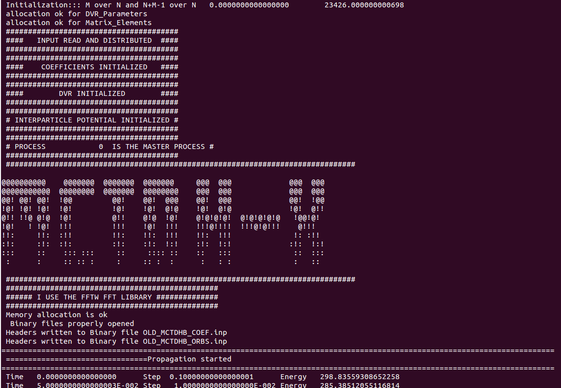
 MCTDHX

. This should show an output similar to the following figure 1.

Figure 1: Output of an MCTDH-X computation in the shell.

This computation is going to take a minute so sit back and relax or just get a coffee, until it finished. The energy you should see on screen in the final propagation step should be identical to 259.14031953. To visualize the output, let's use gnuplot:

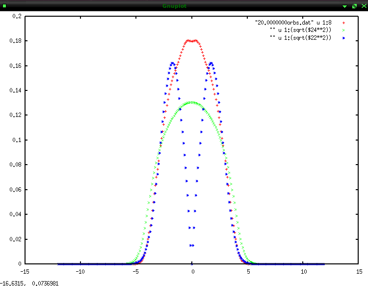
 mctdhx_gnuplot
 plot "20.0000000orbs.dat" u 1:8, "" u 1:(sqrt($24**2)), "" u 1:(sqrt($22**2))

. The plot command visualizes the density $\rho(x)$ (column 8) and the first two natural orbitals $\phi_1^{(NO)}(x)$ and $\phi_2^{(NO)}(x)$ (column 24 and 22, respectively) in the last ASCII output file of the relaxation 20.0000000orbs.dat. For a full explanation of the structure of this file, see table 14. In figure 2, you can see a screenshot of what your gnuplot output should look alike.

Figure 2: Visualization of MCTDH-X relaxation using gnuplot. The density $\rho(x)$ and the first two natural orbitals $\phi_1^{(NO)}(x)$ and $\phi_2^{(NO)}(x)$ are shown as red, green and blue line, respectively.

To find out the occupations of the natural orbitals, let's have a look at the last line of the NO_PR.out file:

 tail -n 1 NO_PR.out

. We get

20.00000000000031 0.5453108642221355E-02 0.1164565131824607E-01 0.2265201507726221E-01 0.9602492249622707 259.1403195319616

which is the time $t$, the natural occupations $\rho_M^{(NO)}(t), \rho_{M-1}^{(NO)}(t),...,\rho_1^{(NO)}(t)$ and the energy of the system $E(t)$, in the final column (see also table 11 for the structure of the NO_PR.out file). We conclude that despite the strong interactions of $\lambda_0=1.0$, our eigenstate of the $N=50$ bosons in the harmonic confinement is close to condensed, since $96\%$ of the bosons sit in the lowest single-particle state. In the single-well, this absence of fragmentation in the groundstate is anticipated. There is, however, numerous examples on the emergence of fragmentation in the dynamics of ultracold bosonic systems. To see the occurence of fragmentation, it's therefore instructive to change the potential in which our eigenstate was computed and trigger some dynamics.