Table 22:
Structure of the <time>N<N>M<M>x-density.dat and <time>N<N>M<M>k-density.dat files.
Column to
Column to
or
or
These files are generated if Density_X/Density_K it true. and
are the spatial and momentum grid, respectively, is the number of internal states, and
and
are the spatial and momentum densities, respectively. In the case of a computation treating atoms with internal structure, the index runs through all internal states of the considered atoms and one density is output for every state.
In the names of the files <time> is the time <N> is the particle number, <M> is the orbital number.
Table 23:
The nonescape probability output file Nonescape.
Column
Column
Time
Nonescape probability
If the input variable Pnot and the borders and were defined with xstart and xend in the input of the analysis program, this file is created.
Table 24:
Structure of the Entropy.dat file.
Column
Column
Column
Column
Time
]
Column
Column
Column
This file is generated when Entropy is set to true. The last column is only present if NBody_C_Entropy=.T. is set in analysis.inp.
Table 25:
Structure of the TwoBody_Entropy.dat file
Column
Column
Column
Column
Time
. This file is generated when TwoBody_Entropy is true.
Table 26:
Structure of the <time>N<N>M<M>x-correlations.dat and <time>N<N>M<M>k-correlations.dat files for multilevel computations.
Column to
Column to
Column
Column &
Column
or
or
or
or
or
Column
or
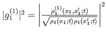
(For the explanation of the filenames, see table 22). These files are created, if the input variable Correlations_X and Correlations_K, respectively, are set to be true. The files contain all necessary quantities to compute the one-body as well as the diagonal of the two-body normalized (Glauber-) correlation function and , respectively, for all internal states . For instance,
can be plotted as the value of ( (Column ) + (Column ) ) divided by (Column ) (Column ).
Table 27:
Structure of the <time>N<N>M<M>x-correlations.dat and <time>N<N>M<M>k-correlations.dat files.
Column to
Column to
Column
Column &
Column
or
or
or
or
or
Column
or
(For the explanation of the filenames, see table 22). These files are created, if the input variable Correlations_X and Correlations_K, respectively, are set to be true. The files contain all necessary quantities to compute the one-body as well as the diagonal of the two-body normalized (Glauber-) correlation function and , respectively. For instance,
can be plotted as the value of ( (Column ) + (Column ) ) divided by (Column )(Column ).
Table 28:
Structure of the <time>N<N>M<M><x/k>corr<1/2>restr.dat files.
Column &
Column &
Column
Column
or
or
or
or
The generation of these files is triggered by the analysis input variables corr1restr,corr2restr,corr1restrmom,corr2restrmom. Similar to the above table 27, the normalized correlation functions and can be computed from the contents of these files, but for one-dimensional computations and on a restricted grid which is specified through the analysis input variables <x/k>ini<1/2>,<x/k>fin<1/2>,<x/k>pts<1/2>, respectively.
Table 29:
Structure of the <time>N<N>M<M>x/k-order-<order>-correlations1D.dat
Column to
Column
Column
Column &
or
or
or
or
(For the explanation of the filenames, see table 22). These files are created, if the input variable anyordercorrelations_X and anyordercorrelations_K as well as oneD, respectively, are set to be true. The files contain all necessary quantities to compute the correlation functions up to order <order>. Here, ///// correspond to the reference point specified in the input file by c_ref_x/c_ref_y/c_ref_z, respectively.
Table 30:
Structure of the CorrelationCoefficient.dat file. This file is created when Correlation_Coefficient it true.
Column
Column &
time
Real & imaginary part of
Table 31:
Structure of the <time>N<N>M<M>x-StructureFactor.dat files. These files are output if StructureFactor is true.
Column to
Column and
Column and
Column to
Column &
Real and imaginary part of
Real and imaginary part of
Real and imaginary part of dynamic structure factor
Table 32:
Structure of the lossops_N2_<border>.dat files.
Column
Column
Column
Column
Time
The generation of such a file is triggered by the lossops input variable being set to .T.. <border> is controlled by the border input variable. For each point in time , a line in this file contains the probability to find particles to the left of border, the probability to find one particle to the left and one to the right of border, and the probability to find two particles to the right of border.
Table 33:
The structure of the <time>N<N>M<M><x/k><Slice 1>-<Slice 2>-correlations.dat files
Column to
Column
Column
Column &
Column
. These are output by the analysis program if the analysis input variable MOMSPACE2D or REALSPACE2D is set to .T.. <Slice 1/2> specify which cut through the real- or momentum-space density are in the file.
Table 34:
The structure of the <time>N<N>M<M><x/k>-SkewCorrelations.dat files
Column and
Column
Column and
Column
Column
. These files are output of the analysis program if the analysis input variable MOMSKEW2D or REALSKEW2D is set to .T. .
Table 35:
The structure of the <time>N<N>M<M><x/k>SingleShots.dat files
Column
Column to
samples of the -body density
. These files are output of the analysis program if the analysis input variable SingleShot_Analysis or SingleShot_FTAnalysis is set to .T. .
Table 36:
The structure of the <time>N<N>M<M><x/k>CentreOfMass.dat files
Column
Column
Histogram of
samples of the centre-of-mass-operator.
. These files are output of the analysis program if the analysis input variable CentreOfMass or CentreOfMomentum is set to .T. .
Table 37:
The structure of the <time>N<N>M<M>phase.dat files.
Column to
Column
Column to
Column &
Column & to &
to
&
&
to
&
The generation of the files is toggled by setting the analysis input variable PHASE to .T.. If additionally GRADIENT it set to .T. then, Columns to containing the phase gradients will be generated. Here are the coordinates,
is the average phase,
to
are the orbital phases,
&
is the and component of the average phase's gradient, and
&
to
&
are the and components of the gradients of the orbital phases.
 can be plotted as the value of ( (Column
 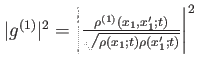 can be plotted as the value of ( (Column
 ![$ S_{\rho_k^{(GO)}}(t)=\sum_i - \frac{\rho^{(GO)}_i(t)}{N} ln [\frac{\rho^{(GO)}_i(t)}{N}] $](img294.png)