Doing the tutorial examples “from scratch”

To prepare the input files in the steps 4. and 6. below, please confer the Tables S1, S2, S3, S4 and S5. These tables illustrate how to modify the default input files included in the MCTDH-X software in order to repeat the simulations that are presented in the main text. For a detailed description of the inputs, refer to the manual at http://ultracold.org/manual.

To run the MCTDH-X software, the following steps are generally taken:

Create a new folder.
Optionally: If you restart your computation from a previous one in the folder <restart-from>, copy the necessary data from there to the working directory:
cp <restart-from>/*bin
cp <restart-from>/Header
Optionally: If you do not restart a previous computation copy the default inputs and executables:
inpcp
bincp
Modify the input file MCTDHX.inp according to your needs (for instance, as indicated in the Tables S1,S2, S3, S4 below).
Run the program: MCTDHX
Configure the analysis task by modifying the file analysis.inp to extract the observables you want (for instance, as indicated in Table S5 below).
Run the analysis: MCTDHX_analysis
Visualize the results using gnuplot or similar. For a detailed description on the structure of the input and output of the MCTDH-X software, please refer to the manual at http://ultracold.org/manual.

For the relaxations, the program (command MCTDHX ) can be directly executed when the executables and the modified input file that contains the Hamiltonian are present in the current working directory. For relaxations, we use randomly generated initial states to circumvent a convergence to excited states. When “repetition” is given as a keyword in a table, the program should be executed multiple ( $\sim$ 10) times with the same input file, and the energies of the resulting states should be compared in order to choose the correct ground state (this applies to problem #10, i.e., Fig. 5(a) and Table S3).

In our simulations of time-evolving states, the initial states are all obtained from relaxations. The results of the relaxations are saved in the binary files PSI_bin, CIc_bin and Header. They should be copied into the folder where propagations are performed. With the input file, binary files, and library in one folder, we can execute the program with the command MCTDHX. We should always verify that the propagations and the corresponding relaxations have compatible input variables like orbital number, particle number, grid size, etc..

There are several input variables for which we provide a more detailed explanation.

The potentials HO1D, HO1D+td_gauss, and HO1D+td_g_r are defined respectively as

$\displaystyle V(x)$ $\displaystyle =$ $\displaystyle \frac{1}{2}p_1^2(x-p_2)^2,\quad \mathtt{HO1D}$ (1)

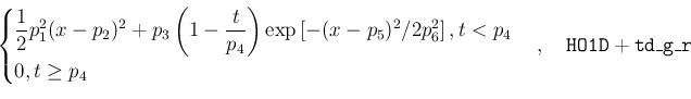
$\displaystyle V(x)$ $\displaystyle =$ $\begin{displaymath}\begin{cases} \dfrac{1}{2}p_1^2(x-p_2)^2 + p_3\dfrac{t}{p_4}\... ...6^2 \right], t\ge p_4 \end{cases},\quad \mathtt{HO1D+td\_gauss}\end{displaymath}$ (2)

$\displaystyle V(x)$ $\displaystyle =$ $\begin{displaymath}\begin{cases} \dfrac{1}{2}p_1^2(x-p_2)^2 + p_3\left(1-\dfrac{... ... t<p_4 \\ 0, t\ge p_4 \end{cases},\quad \mathtt{HO1D+td\_g\_r}\end{displaymath}$ (3)

where is the position, is the imaginary or real time, and to correspond to the input variables parameter1 to parameter6 in the input file MCTDHX.inp, respectively.
The interparticle interaction can be chosen in the following way. The contact interaction can be chosen by setting Interaction_Type = 0. In this case, the variables which_interaction, Interaction_Parameter1, and Interaction_Parameter2 are irrelevant. The regularized Coulomb interaction can be chosen by setting which_interaction = regC, Interaction_Type = 4, and Interaction_Parameter1 and Interaction_Parameter2 are respectively $\alpha$ and $\beta$ in Eq.(14b) in the main text. Other type of interaction can be chosen by using different keywords for which_interaction. Detailed descriptions of these interactions are given in the manual at http://ultracold.org/data/manual
The number of grids NDVR_X is recommended to be a powers of 2.

If you get stuck, you may check the supplied input files and scripts in Sec. S1.2.1 available for download at http://ultracold.org/data/tutorial_input_files.zip and the manual at http://ultracold.org/manual. The structure of the folder tree in tutorial_input_files.zip is explained in Figs. S2,S3,S4, S5, S6, S7and S8.

$\displaystyle V(x)$	$\displaystyle =$	$\displaystyle \frac{1}{2}p_1^2(x-p_2)^2,\quad \mathtt{HO1D}$	(1)
$\displaystyle V(x)$	$\displaystyle =$	$\begin{displaymath}\begin{cases} \dfrac{1}{2}p_1^2(x-p_2)^2 + p_3\dfrac{t}{p_4}\... ...6^2 \right], t\ge p_4 \end{cases},\quad \mathtt{HO1D+td\_gauss}\end{displaymath}$	(2)
$\displaystyle V(x)$	$\displaystyle =$	$\begin{displaymath}\begin{cases} \dfrac{1}{2}p_1^2(x-p_2)^2 + p_3\left(1-\dfrac{... ... t<p_4 \\ 0, t\ge p_4 \end{cases},\quad \mathtt{HO1D+td\_g\_r}\end{displaymath}$	(3)